We have now loaded the full Quarterly Bulletin (QB) vintage history into EconData, from 2004Q3 to the current period, available publicly, for free. This spans 22 years and 85 quarters so far, with about 4600 series. The latest version of our QB datasets is 1.1.4, which is where we loaded the full vintage history recently. Our QB datasets are:
- Money and Banking
QB_MONBANK - Capital Market
QB_CAPMARK - Public Finance
QB_PUBLFIN - External Economic Accounts
QB_BALNPAY - National Accounts
QB_NATLACC - General Economic Indicators
QB_BUSCYCL
(see more details on the user guide page).
Nomenclature
Although each QB is published at the end of each quarter, the vintage description is the previous quarter, as the quarterly data is only up-to-date as of the previous quarter (even though monthly, weekly and daily data is more up-to-date). For example, we named the 30 September 2025 vintage “2025Q2”.
Intra-quarterly updates
In-between each quarterly load, we also query QB series from the SARB’s API, and update the QB with that subset, staging the data every weekday (as “unreleased” in EconData) and releasing that on or after the 10th day of every month.
Evidence of our current set of vintages
Please run the econdatar::read_release("DATASET_ID") function in R, to see the available vintages (with version = "latest" by default). For example,
> read_release("QB_MONBANK")
Fetching releases for: ECONDATA-QB_MONBANK-1.1.4

                release start-period end-period         description
                 <POSc>       <POSc>     <POSc>              <char>
 1: 2026-06-30 10:00:00   1960-01-01 2026-06-12 2026Q1 (2026-06-30)
 2: 2026-03-31 10:00:00   1948-12-01 2026-03-09 2025Q4 (2026-03-31)
 3: 2025-12-31 10:00:00   1948-12-01 2025-11-24 2025Q3 (2025-12-31)
 4: 2025-09-30 10:00:00   1960-01-01 2025-06-13 2025Q2 (2025-09-30)
 5: 2025-06-30 10:00:00   1922-12-01 2025-06-09 2025Q1 (2025-06-30)
 6: 2025-03-31 10:00:00   1922-12-01 2025-03-14 2024Q4 (2025-03-31)
 7: 2024-12-31 10:00:00   1948-12-01 2024-11-29 2024Q3 (2024-12-31)
 8: 2024-09-30 10:00:00   1960-01-01 2024-09-13 2024Q2 (2024-09-30)
 9: 2024-06-30 10:00:00   1960-01-01 2024-06-29 2024Q1 (2024-06-30)
10: 2024-03-31 10:00:00   1964-01-01 2024-03-11 2023Q4 (2024-03-31)
11: 2023-12-31 10:00:00   1964-01-01 2023-12-01 2023Q3 (2023-12-31)
12: 2023-09-30 10:00:00   1960-01-01 2023-09-08 2023Q2 (2023-09-30)
13: 2023-06-30 10:00:00   1960-01-01 2023-06-15 2023Q1 (2023-06-30)
14: 2023-03-31 10:00:00   1964-01-01 2023-03-13 2022Q4 (2023-03-31)
15: 2022-12-31 10:00:00   1964-01-01 2022-11-25 2022Q3 (2022-12-31)
16: 2022-09-30 10:00:00   1922-12-01 2022-09-09 2022Q2 (2022-09-30)
17: 2022-06-30 10:00:00   1922-12-01 2022-06-10 2022Q1 (2022-06-30)
18: 2022-03-31 10:00:00   1948-12-01 2022-03-07 2021Q4 (2022-03-31)
19: 2021-12-31 10:00:00   1960-01-01 2021-11-29 2021Q3 (2021-12-31)
20: 2021-09-30 10:00:00   1922-12-01 2021-09-10 2021Q2 (2021-09-30)
21: 2021-06-30 10:00:00   1948-12-01 2021-06-04 2021Q1 (2021-06-30)
22: 2021-03-31 10:00:00   1960-01-01 2021-03-05 2020Q4 (2021-03-31)
23: 2020-12-31 10:00:00   1948-12-01 2020-07-06 2020Q3 (2020-12-31)
24: 2020-06-30 10:00:00   1960-01-01 2020-07-03 2020Q1 (2020-06-30)
25: 2020-03-31 10:00:00   1960-01-01 2020-02-28 2019Q4 (2020-03-31)
26: 2019-12-31 10:00:00   1964-01-01 2019-11-22 2019Q3 (2019-12-31)
27: 2019-09-30 10:00:00   1960-01-01 2019-08-26 2019Q2 (2019-09-30)
28: 2019-06-30 10:00:00   1960-01-01 2019-05-27 2019Q1 (2019-06-30)
29: 2019-03-31 10:00:00   1948-12-01 2019-03-01 2018Q4 (2019-03-31)
30: 2018-12-31 10:00:00   1948-12-01 2018-11-30 2018Q3 (2018-12-31)
31: 2018-09-30 10:00:00   1960-01-01 2018-08-13 2018Q2 (2018-09-30)
32: 2018-06-30 10:00:00   1964-01-01 2018-05-18 2018Q1 (2018-06-30)
33: 2018-03-31 10:00:00   1964-01-01 2018-02-19 2017Q4 (2018-03-31)
34: 2017-12-31 10:00:00   1960-01-01 2017-10-30 2017Q3 (2017-12-31)
35: 2017-09-30 10:00:00   1960-01-01 2017-08-18 2017Q2 (2017-09-30)
36: 2017-06-30 10:00:00   1960-01-01 2017-05-19 2017Q1 (2017-06-30)
37: 2017-03-31 10:00:00   1960-01-01 2017-02-24 2016Q4 (2017-03-31)
38: 2016-12-31 10:00:00   1960-01-01 2016-11-11 2016Q3 (2016-12-31)
39: 2016-09-30 10:00:00   1960-01-01 2016-08-08 2016Q2 (2016-09-30)
40: 2016-06-30 10:00:00   1922-12-01 2016-05-06 2016Q1 (2016-06-30)
41: 2016-03-31 10:00:00   1960-01-01 2016-01-25 2015Q4 (2016-03-31)
42: 2015-12-31 10:00:00   1922-12-01 2015-11-06 2015Q3 (2015-12-31)
43: 2015-09-30 10:00:00   1960-01-01 2015-08-03 2015Q2 (2015-09-30)
44: 2015-06-30 10:00:00   1960-01-01 2015-05-08 2015Q1 (2015-06-30)
45: 2015-03-31 10:00:00   1960-01-01 2015-02-06 2014Q4 (2015-03-31)
46: 2014-12-31 10:00:00   1960-01-01 2014-11-07 2014Q3 (2014-12-31)
47: 2014-09-30 10:00:00   1948-12-01 2014-08-08 2014Q2 (2014-09-30)
48: 2014-06-30 10:00:00   1960-01-01 2014-05-05 2014Q1 (2014-06-30)
49: 2014-03-31 10:00:00   1922-12-01 2014-02-03 2013Q4 (2014-03-31)
50: 2013-12-31 10:00:00   1922-12-01 2013-10-28 2013Q3 (2013-12-31)
51: 2013-09-30 10:00:00   1948-12-01 2013-08-12 2013Q2 (2013-09-30)
52: 2013-06-30 10:00:00   1960-01-01 2013-05-06 2013Q1 (2013-06-30)
53: 2013-03-31 10:00:00   1960-01-01 2012-12-01 2012Q4 (2013-03-31)
54: 2012-12-31 10:00:00   1948-12-01 2012-11-12 2012Q3 (2012-12-31)
55: 2012-09-30 10:00:00   1948-12-01 2012-08-06 2012Q2 (2012-09-30)
56: 2012-06-30 10:00:00   1960-01-01 2012-04-30 2012Q1 (2012-06-30)
57: 2012-03-31 10:00:00   1960-01-01 2012-02-06 2011Q4 (2012-03-31)
58: 2011-12-31 10:00:00   1960-01-01 2011-11-14 2011Q3 (2011-12-31)
59: 2011-09-30 10:00:00   1960-01-01 2011-08-15 2011Q2 (2011-09-30)
60: 2011-06-30 10:00:00   1960-01-01 2011-05-09 2011Q1 (2011-06-30)
61: 2011-03-31 10:00:00   1960-01-01 2011-02-21 2010Q4 (2011-03-31)
62: 2010-12-31 10:00:00   1960-01-01 2010-09-18 2010Q3 (2010-12-31)
63: 2010-09-30 10:00:00   1948-12-01 2010-08-16 2010Q2 (2010-09-30)
64: 2010-06-30 10:00:00   1960-01-01 2010-05-03 2010Q1 (2010-06-30)
65: 2010-03-31 10:00:00   1960-01-01 2009-12-28 2009Q4 (2010-03-31)
66: 2009-12-31 10:00:00   1960-01-01 2009-10-05 2009Q3 (2009-12-31)
67: 2009-09-30 10:00:00   1948-12-01 2009-07-20 2009Q2 (2009-09-30)
68: 2009-06-30 10:00:00   1960-01-01 2009-05-04 2009Q1 (2009-06-30)
69: 2009-03-31 10:00:00   1948-12-01 2009-02-16 2008Q4 (2009-03-31)
70: 2008-12-31 10:00:00   1960-01-01 2008-10-27 2008Q3 (2008-12-31)
71: 2008-09-30 10:00:00   1960-01-01 2008-08-04 2008Q2 (2008-09-30)
72: 2008-06-30 10:00:00   1960-01-01 2008-04-21 2008Q1 (2008-06-30)
73: 2008-03-31 10:00:00   1960-01-01 2008-02-11 2007Q4 (2008-03-31)
74: 2007-12-31 10:00:00   1948-12-01 2007-11-12 2007Q3 (2007-12-31)
75: 2007-09-30 10:00:00   1960-01-01 2007-08-13 2007Q2 (2007-09-30)
76: 2007-06-30 10:00:00   1960-01-01 2007-03-01 2007Q1 (2007-06-30)
77: 2007-03-31 10:00:00   1964-01-01 2007-02-12 2006Q4 (2007-03-31)
78: 2006-12-31 10:00:00   1964-01-01 2006-11-06 2006Q3 (2006-12-31)
79: 2006-09-30 10:00:00   1960-01-01 2006-08-14 2006Q2 (2006-09-30)
80: 2006-06-30 10:00:00   1960-01-01 2006-06-01 2006Q1 (2006-06-30)
81: 2006-03-31 10:00:00   1960-01-01 2006-08-14 2005Q4 (2006-03-31)
82: 2005-12-31 10:00:00   1960-01-01 2006-08-14 2005Q3 (2005-12-31)
83: 2005-09-30 10:00:00   1960-01-01 2006-06-01 2005Q2 (2005-09-30)
84: 2005-06-30 10:00:00   1960-01-01 2005-05-23 2005Q1 (2005-06-30)
85: 2005-03-31 10:00:00   1960-01-01 2005-02-21 2004Q4 (2005-03-31)
86: 2004-12-31 10:00:00   1960-01-01 2004-11-15 2004Q3 (2004-12-31)
                release start-period end-period         description
This looks the same for
read_release("QB_CAPMARK")
read_release("QB_PUBLFIN")
read_release("QB_BALNPAY")
read_release("QB_NATLACC")
read_release("QB_BUSCYCL")
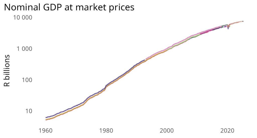
Comparing series over vintages
You can compare a series over all the vintages with the hist_obs option when extracting the data. The following code produces the plot below it, with each colour representing data from a different vintage.
library(econdatar)
library(tidyverse)
library(hues)

data_qb_history <- read_dataset(
    id = "QB_NATLACC",
    tidy = FALSE,
    wide = FALSE,
    combine = TRUE,
    series_key = "KBP6006L.Q.N.S.LA",
    hist_obs = TRUE
)

ggplot_history <- ggplot(data_qb_history[["KBP6006L.Q.N.S.LA"]] %>%
        as_tibble() %>%
        mutate(created = format(ymd_hms(created), "%Y-%m-%d"),
            TIME_PERIOD = ymd(TIME_PERIOD)) %>%
        complete(created, TIME_PERIOD),
    aes(x = TIME_PERIOD, colour = created, y = OBS_VALUE / (10^3))) +
geom_line(
    linewidth = rel(0.65),
    alpha = 0.75,
    show.legend = FALSE
) +
theme_minimal() +
scale_y_log10(
    labels = scales::label_number(big.mark = " ")
) +
theme(
    axis.title.x = element_blank(),
    legend.text = element_text(size = rel(0.6)),
    legend.key.spacing.y = unit(-0.3, "lines"),
    plot.title.position = "plot",
    panel.grid = element_blank()
) +
labs(
    y = "R billions",
    title = "Nominal GDP at market prices",
    colour = "Vintage"
) +
scale_color_manual(
    values = iwanthue(n = length(unique(data_qb_history[[1]]$created)))
)

ggsave(
    file = "sarb/qb/gdp_history.jpg",
    plot = ggplot_history,
    width = 13,
    height = 7,
    unit = "cm"
)
By Aidan Horn, data engineer @ Codera Analytics