Charting and automation

Most economists and other data professionals spend a lot of time creating interesting and insightful data visualisations. Unfortunately, just as many spend perhaps even more time updating their charts or recreating the charts of others.

A key feature of EconData is to allow you to create charts and visualisations that are easily updated or repurposed.

In this blog post, we illustrate how to import data into R using EconData and how to create a simple chart. The idea is to provide a starting point that can be used for automated plotting. The source code can be found here.

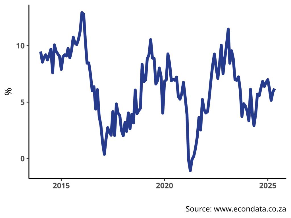
Example: Growth in total loans and advances in South Africa (year-on-year)

The first step towards automating a chart is setting up your own template. In your template you should include with the data series that you would like to see on an ongoing basis, and change the plotting instructions to reflect your preferred chart format. Thereafter, all that is required is to run the script any time you would like to see the latest plots of the data.

Let’s take it step by step. First, lets load the required R packages.

library(econdatar)
library(dplyr)
library(ggplot2)
library(gridExtra)

Note the inclusion of the EconData package library(econdatar). Since this package is available on Github and not yet on CRAN you will not be able to install it in the typical way. The easiest way to install the EconData R package is by running the following.

install.packages("remotes", 
                 repos = "https://cran.mirror.ac.za")
library("remotes")
install_github("coderaanalytics/econdatar")

Using the read_dataset() function, we can import the data directly into R. In order to use the function, you will need an active account with EconData, which can be created by clicking on “Sign up” at the bottom of the sign-in screen of the app.

Note: In order to use econdatar functions in R, a username and password are required. This dialogue box will be active when the function runs but the window may not pop up. Please check your task bar for the window, to fill in your credentials.

ba100 <- read_dataset(id = "BA100",
                      series_key = "TOT..L024")

The function requires, at a minimum, that the data set ID be provided—in this case the BA100 data set. We also specify the series key so that only the time series that we are interested in be returned. The data we are downloading for this tutorial is total credit extension from all banking institutions in South Africa, which has the data key of TOT.A3.L024.

Next, let’s take a look at how the data key is constructed for those that are interested. This next paragraph can be skipped without loss of continuity.

The series key refers to the searchable dimensions of the data set. TOT is the first dimension, which represents the bank in question; here specifically it is the aggregation for all the banks in South Africa, the grand total. A3 is the second dimension, which represents a column, or aggregation, of a table in the BA100 form—here again it is the total. And lastly, L024 is the third dimension, and it represents the 24th line of the BA100 form, namely gross loans and advances. Leaving out any dimension acts as a wildcard for that dimension, for example, the data key TOT..L024 will return all aggregations of the BA100 form matching the two given dimensions. A good way of getting the hang of how this works, is to play with the EconData web app. Pay specific attention to the export functionality and the generated R code. We go deeper into the details of the read_dataset() function here. Help on the function is also available in R using the command ?read_dataset.

In the wide format that we downloaded (by default), some simple metadata such as the series names are included, shown in the following two lines of code.

attributes(ba100)$metadata
attributes(ba100$TOT.A3.L024)

(To see the full set of metadata, rather specify the option wide = FALSE in the read_dataset() function.)

Next, using some functions from the dplyr package, we can convert the time series data to a tibble format which allows for easy data manipulation and plotting. Also using dplyr, we are converting the raw data to a year-on-year growth rate.

loans_and_advances <- as_tibble(ba100) %>%
    arrange(time_period) %>%
    mutate(growth = (TOT.A3.L024 / dplyr::lag(TOT.A3.L024, n = 12) - 1) * 100) %>%
    filter(!is.na(growth))

Lastly, using the ggplot2 package we can create a simple line plot to visualise the data.

p <- ggplot(data = loans_and_advances) +
  geom_line(aes(x = time_period, y = growth), colour = "#273b8d", linewidth = 2) +
  labs(caption = "Source: www.econdata.co.za") +
  xlab("") + ylab("%") +
  theme_classic(base_size = 14) +
  theme(panel.grid = element_blank(),
        axis.text = element_text(face = "bold"))

The Codera Analytics team