Apart from automating your charts, EconData makes it possible for you to automate your models. Model automation is usually not a trivial thing to do. But EconData’s functionality and its integration into R makes this easy. In this blog post, we illustrate how to create a naïve automated forecasting model using EconData.
The specification of the model is handled by the R forecast package, which employs an algorithm to choose an ARIMA model that best fits the data. All that is required to estimate the model and produce an updated forecast is to run the script.
In today’s example, we will load historical Headline CPI data, produce a plot and then produce a forecast. We start by creating a new script and running the following to load the required packages.
library(remotes)
install_github("coderaanalytics/econdatar")
library(econdatar)
Next, load the required packages. A previous tutorial on installing the EconData package.
library(econdatar)
library(magrittr)
library(forecast)
library(xts)
library(gridExtra)
library(dplyr)
We can now load the data using the read_econdata() function. Specify the data set id, data key, and releasedescription.
cpi <- read_econdata(id = "CPI_COICOP_5",
                     key = "TC.00.0.0.0",
                     releasedescription = "latest")
In this post, we focus on the releasedescription argument of the read_econdata() function. This next section can be skipped without loss of continuity.
Each data set available on the EconData has multiple releases. Each release corresponds to a snapshot of the data as was available at the time of the release, sometimes referred to as a ‘data vintage’. By making it easy to access historical data vintages, EconData enables easy testing of the real-time performance of a model. This is very important for modelling economic data that get revised, such as estimating the output gap using GDP data. In order to query the available releases, we use the read_release() function.
read_release(id = "CPI_COICOP_5",
             tidy = TRUE) %>%
    bind_rows()
We must, at a minimum, specify the data set id whose releases we want returned, i.e. read_release(id = "CPI_COICOP_5"). Each release will have a release description which we pass to read_econdata() in order to return the data for that release. If no releasedescription argument is passed to read_econdata(), the latest unreleased data will be returned. If the releasedescription is equal to "latest" the latest release will be returned. We will delve deeper into the workings of EconData’s system for cataloging and identification of data in the next post.
To ease manipulation of the data, we will convert the input data into xts format.
headline <- xts(cpi$TC.00.0.0.0,
                order.by = rownames(cpi$TC.00.0.0.0) %>%
            as.Date() %>%
            as.yearmon())
Next, we can convert the headline CPI data into a year-on-year inflation rate, and plot the data to have a better idea of how to proceed with modeling and forecasting.
headline_yoy <- (headline / stats::lag(headline, k = 12) - 1) * 100

# Open the graphics device
png("CPIforecast.png",
    width = 1200,
    height = 700,
    res = 160)
plot(headline_yoy, main="Headline y-o-y inflation", col="#273b8d", lwd=3)
We are now able to estimate the model. We are using a a simple ARIMA model using the forecast package. The auto.arima() function from the package will automatically choose the model specification that best fits the data.
arima_mod <- auto.arima(headline_yoy)
Now that we have an estimated ARIMA model, we can use the model to forecast. In this example, we are forecasting 12 months ahead.
f_cast <- forecast(arima_mod, h=12)
The forecasts, along with associated confidence intervals, can now be summarised in a plot or table.
plot(f_cast, main = "Forecast of 12-month ahead y-o-y headline inflation",
     col = "#273b8d",
     lwd = 3)

last_date <- last(index(headline_yoy))+1/12
f_cast_data <- data.frame((seq(as.Date(last_date), length=12, by="month")+1),
                f_cast$mean[1:12])
colnames(f_cast_data) <- c("Date","Forecast")
dev.off() # close graphics device

print(f_cast_data)
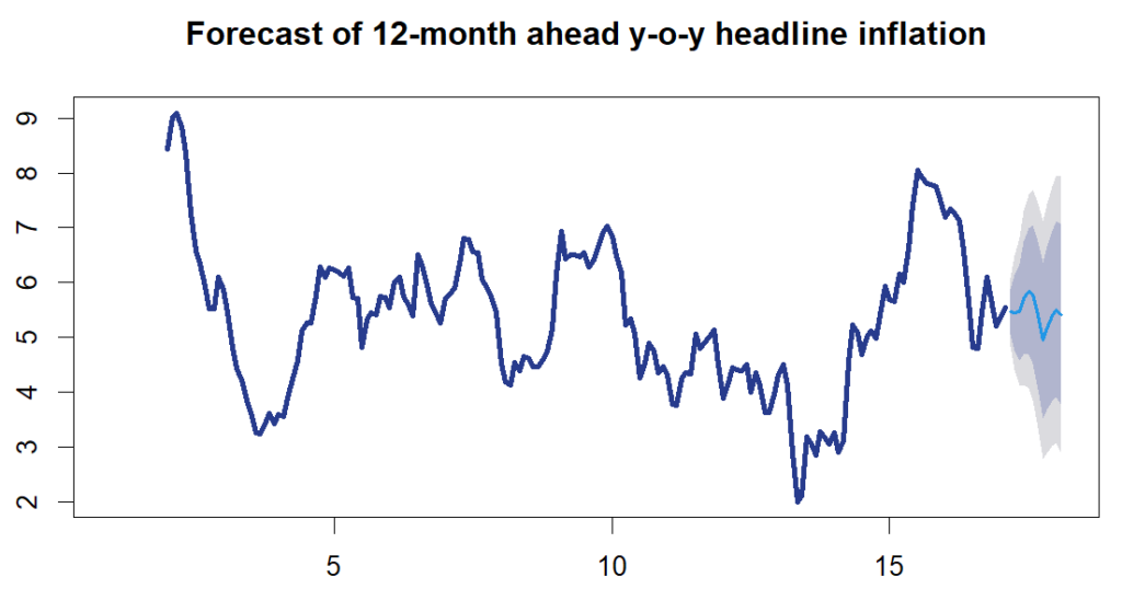
Table of forecasts
| Date | Forecast |
|---|---|
| 2024-03-02 | 5.461227 |
| 2024-04-02 | 5.449294 |
| 2024-05-02 | 5.462961 |
| 2024-06-02 | 5.713285 |
| 2024-07-02 | 5.837858 |
| 2024-08-02 | 5.781177 |
| 2024-09-02 | 5.406796 |
| 2024-10-02 | 4.942001 |
| 2024-11-02 | 5.165841 |
| 2024-12-02 | 5.383796 |
| 2025-01-02 | 5.511582 |
| 2025-02-02 | 5.415028 |
The Codera Analytics team
#ARIMA #automation #modelling #plotting #Tutorial